Example: Auto MPG Analysis with Grid Search

This page walks through a complete causal analysis workflow in Tetrad using the Auto MPG dataset.
It illustrates how to move from data exploration to model selection using Grid Search and Markov checking, following the default workflow recommended in this manual.

The goal is not to identify a single “true” causal graph, but to show how to arrive at a minimal, Markov-consistent model under clearly stated assumptions.

1. The Auto MPG Dataset

We use the Auto MPG dataset from the CMU causal datasets repository:

Repository:
https://github.com/cmu-phil/example-causal-datasets
Data file used:

real/auto-mpg/data/auto-mpg.data.mixed.max.3.categories.txt

Data Preparation

Before loading the data into Tetrad, we made two simple preprocessing decisions:

Removed the car name field, which serves as an identifier and is not meaningful for causal modeling.
Removed rows with missing values, to keep the example focused on the core workflow rather than missing-data handling.

The resulting dataset contains:

Several continuous variables (e.g., mpg, weight, horsepower)
One discrete variable (origin) with three categories

Because of this mixture, the data should be loaded as mixed data with a maximum of 3 categories, as indicated in the file name.

2. Loading and Exploring the Data in Tetrad

Load the dataset into a Data box.
Specify that the data are mixed, with a maximum of 3 categories.

Visual Exploration

Using the Plot Matrix tool in the Data box, we observe:

Strong, approximately linear relationships among many pairs of variables
No obvious nonlinear clusters or sharp discontinuities
Patterns consistent with additive, roughly Gaussian noise

These observations suggest that linear-Gaussian modeling assumptions are reasonable for this dataset, even though one variable is discrete.

3. Algorithm Choice and Assumptions

Causal Sufficiency

For this example, we assume causal sufficiency:

All major common causes of the measured variables are assumed to be observed.
We therefore search for a CPDAG (a Markov equivalence class of DAGs), rather than a PAG.

This is a modeling assumption made for illustration purposes; it simplifies the workflow and is reasonable for this dataset.

Algorithm: BOSS

We choose BOSS, a score-based search algorithm, because:

It performs well in linear settings
It scales well for systematic exploration
It integrates naturally with score-based model comparison

Score: Degenerate Gaussian BIC

Based on data exploration, we select the Degenerate Gaussian BIC score:

It is appropriate for mixed data
It aligns with the approximately linear structure seen in the plot matrix
It supports Markov checking via the DG-LRT test

4. Setting Up the Grid Search

Step 1: Connect the Data

Draw an edge from the Auto MPG Data box to a Grid Search box.

This configures Grid Search to operate directly on the dataset.

Step 2: Algorithms Tab

Go to the Algorithms tab.
Click Add Algorithm.
Select BOSS.
Choose Degenerate Gaussian BIC as the score.

At this point, leave parameter ranges unchanged.

Step 3: Table Columns Tab

Go to the Table Columns tab.
Click Add Table Column(s).
In the dialog, click Markov Check Columns.

Note: At present, there is a UI issue that requires scrolling to the bottom of the dialog to ensure all relevant columns are selected.
(This will be addressed in a future release.)

Click Add.

The selected Markov-check statistics should now appear in the table-columns list.

Step 4: Comparison Tab (Initial Setup)

In the Comparison tab:

Set Comparison Graph Type to CPDAG
Set Sort by Utility to Yes
Set Markov Checker Test to
DG-LRT (Degenerate Gaussian Likelihood Ratio Test)

If you open Edit Utilities, you will see that default utilities for the Markov-check statistics are already configured.

Step 5: Set Parameter Ranges

Return to the Algorithms tab:

Click Edit Parameters
Open the Scores section
For Penalty Discount, enter:

1, 1.2, 1.4, 1.6, 1.8, 2, 2.2, 2.4, 2.6, 2.8, 3, 3.2, 3.4, 3.6

This range spans models from relatively dense to relatively sparse.

5. Running the Comparison

Go back to the Comparison tab.
Click Run Comparison.

Grid Search will:

Run BOSS for each penalty-discount value
Compute Markov-check statistics for each resulting CPDAG
Summarize the results in a comparison table

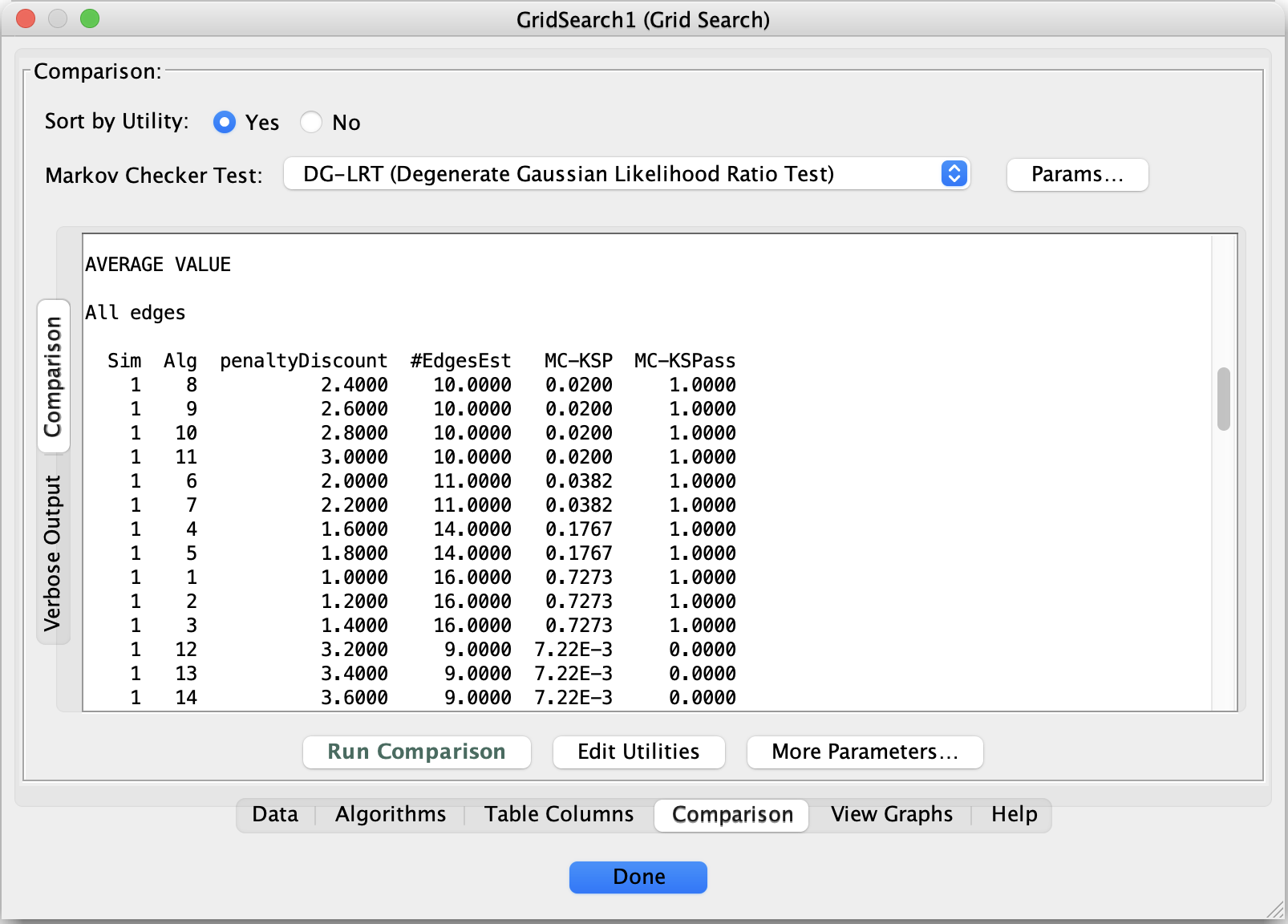
6. Interpreting the Comparison Results

In the comparison table, two columns are especially informative:

MC-KSPass
Indicates whether the model passes the Markov check
#EdgesEst
Indicates model complexity

A common pattern is visible:

Very sparse models fail Markov checking
Very dense models pass but are difficult to interpret
Several intermediate models pass Markov checks

Choosing a Model

Among the rows where MC-KSPass = 1, select the model with the fewest edges.

In this example, that corresponds to:

Algorithm = 8

This choice represents a minimal Markov-consistent CPDAG under the stated assumptions.

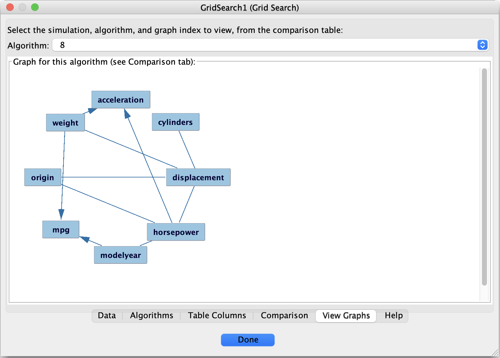
7. Viewing the Selected Graph

Open the View Graphs tab.
Select Algorithm = 8.

The displayed graph is the final candidate model for this analysis.

8. What This Example Illustrates

This worked example demonstrates a complete default workflow in Tetrad:

Explore the data visually
Make assumptions explicit
Use Grid Search to explore parameter sensitivity
Evaluate models using Markov checking
Select a minimal model that passes diagnostics

9. Next Steps

From here, you might:

Explore alternative assumptions (e.g., allowing latent variables)
Inspect Markov-check violations in more detail
Incorporate background knowledge and rerun the analysis
Use the selected structure for causal effect estimation