Detail: SEM (Linear) Estimator
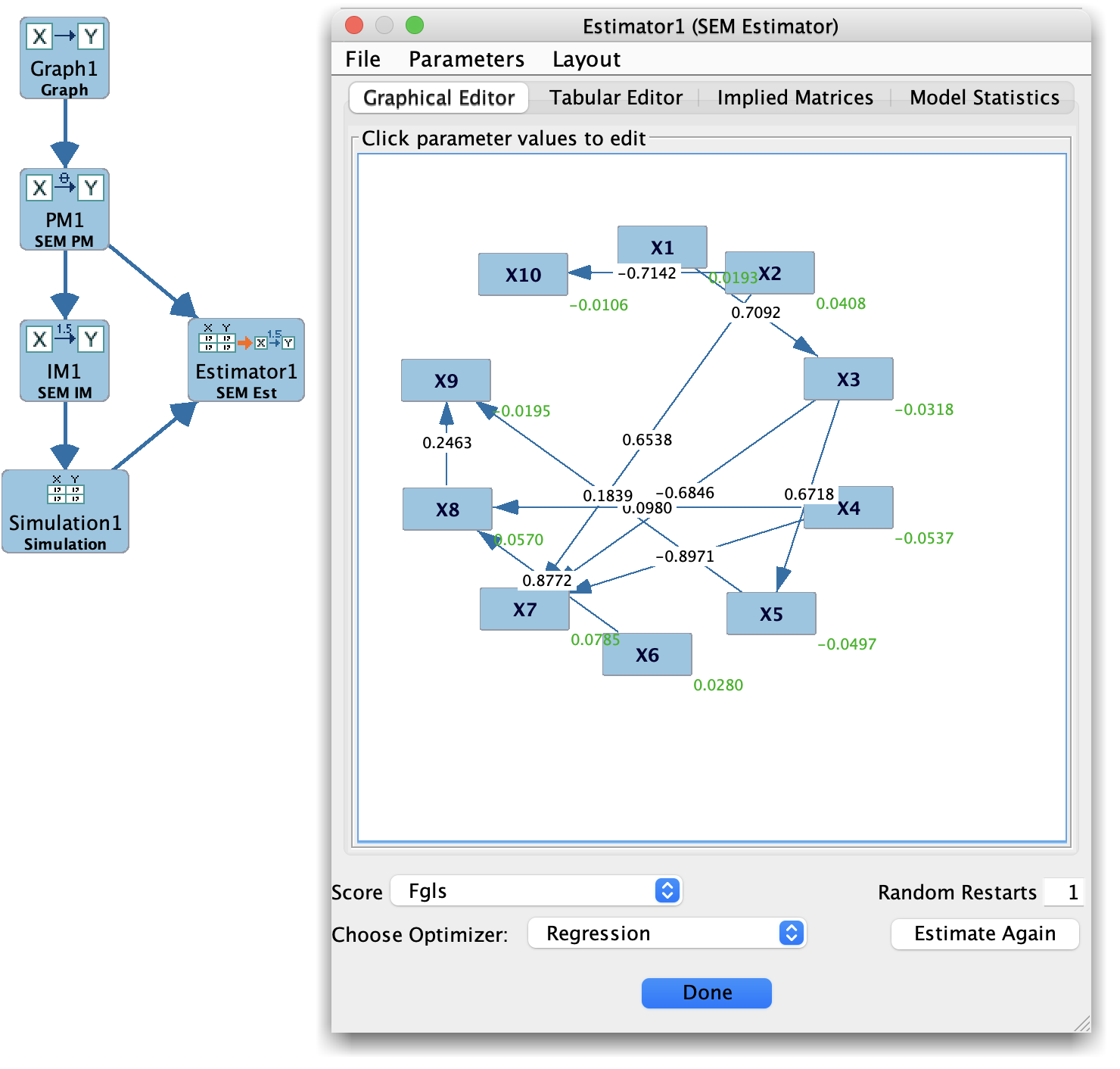
The SEM (Linear) Estimator fits a Structural Equation Model (SEM) Parametric Model to continuous data, assuming linear relations with Gaussian errors. It produces parameter estimates (path coefficients, variances, and possibly means) and global fit statistics.
This estimator is available when the Parametric Model connected to the Estimator box is a SEM PM.
SEM Estimator
Purpose
Estimate:
Regression/path coefficients between variables.
Error variances and possibly covariances.
Optionally, intercepts/means (depending on model specification).
Provide model fit statistics such as:
χ², degrees of freedom, and p-value.
Additional indices like RMSEA, CFI, TLI, BIC (when available).
Inputs and requirements
Parametric Model: A SEM PM specifying:
Directed edges (structural equations),
(Optional) latent variables and measurement relations.
Data:
Continuous measurements aligned with observed variables in the SEM.
Sufficient sample size and variance structure for identification.
Estimation options (when exposed), e.g.:
Handling of means (with or without mean structure).
Missing-data method (e.g., listwise deletion, FIML).
Optimization tolerance and maximum iterations.
Robust corrections (if supported).
How it works (conceptually)
The SEM (Linear) Estimator typically:
Constructs an implied covariance (and mean) model from the SEM PM.
Finds parameters that minimize a discrepancy function between:
the observed sample covariance (and mean) structure, and
the model-implied covariance (and mean) structure.
Uses numerical optimization (e.g., ML-based) to obtain parameter estimates and compute fit statistics.
Output
Parameter table showing:
Path coefficients (regression weights).
Error variances and (where applicable) covariances.
Standard errors and test statistics (if available).
Fit indices:
χ², df, p-value.
Additional indices (RMSEA, CFI, TLI, BIC, etc.), depending on the implementation.
Convergence information and any warnings (e.g., non-positive definite covariance, Heywood cases).
The result can be stored as an Instantiated Model (SEM) for later use.