Estimate model parameters

In many workflows, you do not just want a graph; you also want numerical parameters: regression coefficients, error variances, factor loadings, or conditional probability tables. In Tetrad, these are obtained using the Estimator box, often in combination with Parametric Model and Instantiated Model boxes.

A typical pattern is:

1. Specify a graph that encodes the causal or measurement structure.

2. Choose a model family (Bayes, SEM, Hybrid, Generalized) in a Parametric Model box.

3. Attach an Estimator box to both the model and the data.

4. Run the Estimator to produce an Instantiated Model with fitted parameters and fit statistics.

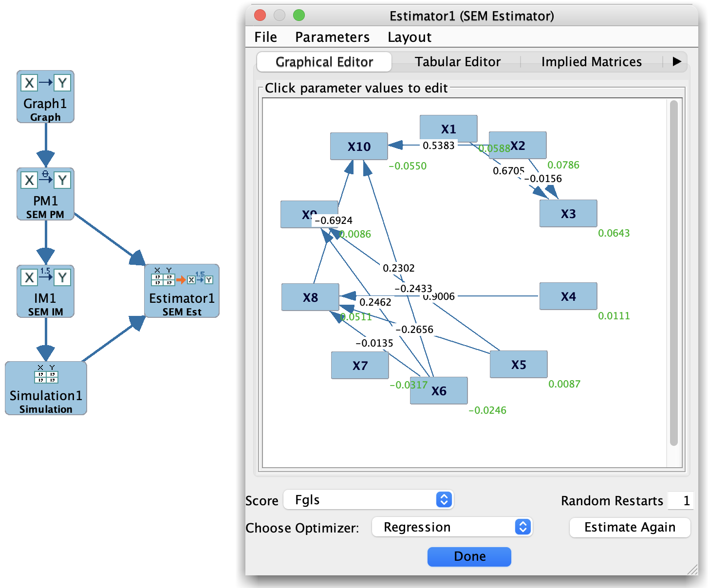
Basic workflow

1. Prepare data

   Make sure you have an appropriate Data or Simulation node in the project tree:

   • Continuous, discrete, or mixed, depending on the model family.

   • Cleaned and typed correctly (variable types set as needed).

2. Specify the model structure

   There are two common starting points:

   • From a graph Use a Graph box to define the structure (DAG, measurement model, etc.), then connect it to a Parametric Model box and select a model family:

     • Bayes (multinomial),

     • SEM (linear SEM),

     • Hybrid (conditional Gaussian),

     • Generalized (user-specified functions and error distributions).

   • From an existing model family If you already have a Parametric Model box configured, you can skip directly to connecting it to an Estimator.

3. Attach an Estimator box

   On the workbench:

   • Place an Estimator box.

   • Connect it to:

     • The Parametric Model (or Graph, for certain estimators that derive parameters directly from a graph), and

     • The appropriate Data or Simulation box.

   The Estimator box now knows:

   • What structure to assume (from the model),

   • What data to use for fitting parameters.

4. Configure and run the estimator

   Double-click the Estimator box to open its configuration dialog. There you can:

   • Choose the estimation method (e.g., SEM Estimator, Bayesian estimator, etc., depending on the model type).

   • Set any estimator-specific options:

     • Handling of missing data,

     • Optimization settings (maximum iterations, convergence criteria),

     • Regularization or constraints, where applicable.

   Click Run to fit the model. When estimation completes, the Estimator box typically produces:

   • An Instantiated Model node (with fitted parameters),

   • Optionally, fit indices and diagnostic tables.

Inspecting the fitted model

Double-click the resulting Instantiated Model node to open it:

• For SEM models, you will see:

  • Estimated path coefficients,

  • Error variances and covariances,

  • Fit indices (e.g., chi-square, CFI, RMSEA, BIC), depending on the estimator.

• For Bayes models, you will see:

  • Conditional probability tables (CPTs) for each variable given its parents.

• For Hybrid / Generalized models, you will see:

  • The parameters appropriate to the chosen family (e.g., conditional Gaussian components, basis-function coefficients, or user-defined functions).

From the Instantiated Model view, you can:

• Inspect parameter values and standard errors (where provided).

• Export parameter tables for use in external software.

• Use the fitted model as input to other boxes:

  • Simulation (to generate new data from the fitted model),

  • Updater (to compute conditional distributions given evidence and interventions),

  • Compare (to evaluate fit or compare fitted models).

Relationship to graphs and search

Estimating model parameters typically comes after you have either:

• Selected a graph structure by hand in the Graph Editor, or

• Learned a graph using a Search box (PC, FGES, GFCI, FCIT, etc.), and then used that learned graph as the basis for a parametric model.

A common end-to-end pipeline looks like:

1. Data → Search → Graph Learn a graph structure from data.

2. Graph → Parametric Model → Estimator → Instantiated Model Choose a model family and estimate parameters.

3. Instantiated Model → Simulation / Updater / Compare Use the fitted model for prediction, simulation, or effect estimation.

This separation—first structure, then parameters—allows you to:

• Compare multiple candidate graphs using the same estimation method.

• Compare multiple model families (e.g., SEM vs Hybrid) on the same graph.

• Re-estimate parameters on new data without changing the underlying structure.

Where to look next

For details on specific estimators and their options, see:

• Estimator Box (box-by-box section),

• Detail: SEM Estimator,

• Parametric Model and Instantiated Model pages for each model family.