Detail: SEM (Linear) Instantiated Model

This page describes SEM (linear) instantiated models in the Instantiated Model box. These are linear Gaussian structural equation models that have been fitted to data, starting from a SEM parametric model.

SEM Instantiated Model

SEM Instantiated Model

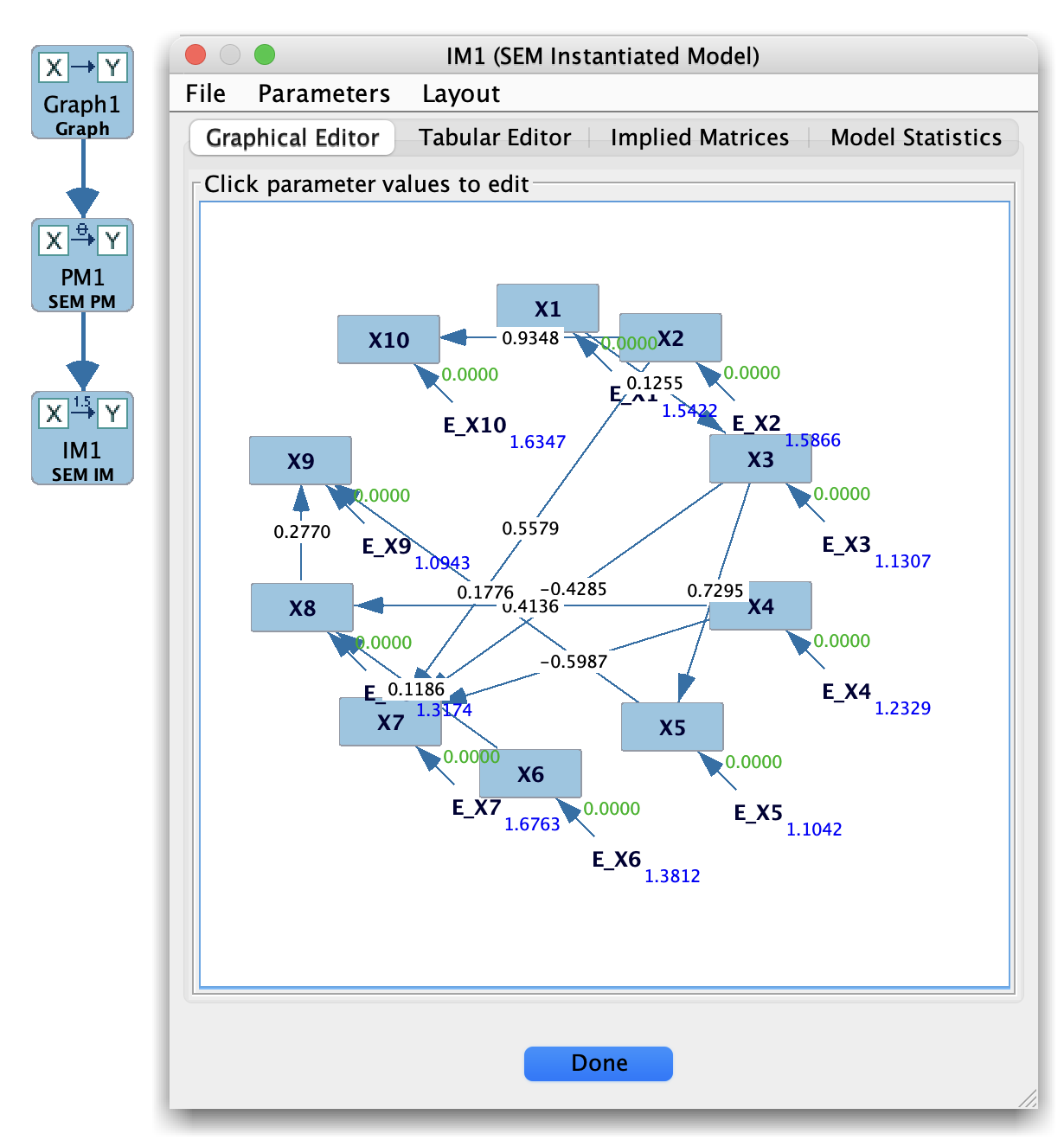
An instantiated SEM model contains:

  • A graph structure (often a DAG or SEM-style graph).

  • Estimated path coefficients for each directed edge.

  • Estimated error variances (and possibly covariances).

  • A set of global fit indices and diagnostics, when available.

How SEM instantiated models are created

  1. In the Parametric Model box, create a SEM (linear) model whose structure matches the SEM graph you want to test.

  2. In the Estimator box, select:

    • The SEM parametric model, and

    • A continuous dataset (from the Data box).

  3. Choose a SEM estimator (e.g., maximum likelihood).

  4. Run the estimator; the result is a fitted SEM.

  5. Save or send this fitted result to the Instantiated Model box.

Each instantiated SEM is tied to a particular dataset and estimation run.

Instantiated Model box layout (SEM)

When you select a SEM instantiated model, the main panel typically displays:

  • A parameter table with:

    • Estimated regression/path coefficients.

    • Standard errors and test statistics (when computed).

    • Estimated error variances (and covariances if allowed).

  • Global fit measures, such as:

    • (\chi^2) and degrees of freedom.

    • RMSEA, CFI, SRMR, BIC, and related indices (depending on implementation).

  • Possibly residual information, such as:

    • Residual covariance matrices.

    • Modification indices (in some versions).

This view is read-only with respect to the estimates; to change the model or estimator you return to the Parametric Model and Estimator boxes.

File menu options (SEM instantiated model)

The File menu of a SEM instantiated model provides several ways to export or reuse the fitted model:

  • Save Graph Image…
    Saves an image of the SEM path diagram to a file. This is useful for including the fitted model in papers, slides, or reports.

  • Copy Implied Covariance Matrix
    Copies the model-implied covariance matrix (\hat\Sigma) of the fitted SEM to the system clipboard as tabular text. You can paste this directly into a spreadsheet, R, Python, or another program.

  • Copy Coefficient Matrix
    Copies the matrix of regression/path coefficients (often called the coefficient or (B) matrix) to the clipboard as tabular text.

  • Copy Error Covariance Matrix
    Copies the residual/error covariance matrix (often called the (\Omega) matrix) to the clipboard as tabular text.

  • Save SEM as XML
    Saves the instantiated SEM in Tetrad’s XML format, including the graph structure, parameter values, and error (co)variances. This is the canonical machine-readable representation and can be reloaded by Tetrad or converted by external tools.

  • Save SEM as Lavaan
    Saves the instantiated SEM as lavaan model syntax in a .lav file.
    When you choose this option, a small dialog lets you select:

    • Whether to include intercepts (lines of the form Y ~ c*1),

    • Whether to include residual variances (Y ~~ v*Y),

    • Whether to include residual covariances (Y ~~ c*Z),

    • And whether to fix parameters to their current values or export them as lavaan start() values for re-estimation.

    The resulting .lav file can be read directly in R using the lavaan package, for example:

    model <- readLines("sem-im.lav")
    fit   <- lavaan::sem(model, data = mydata)